
Hello dear friends, ready for this week’s tip? Today we’ll be continuing the mini-series about investigating the life-cycle of digital images, specifically revealing previous JPEG compressions with Amped Authenticate. If you missed the first tip, it’s here for you. Keep reading.
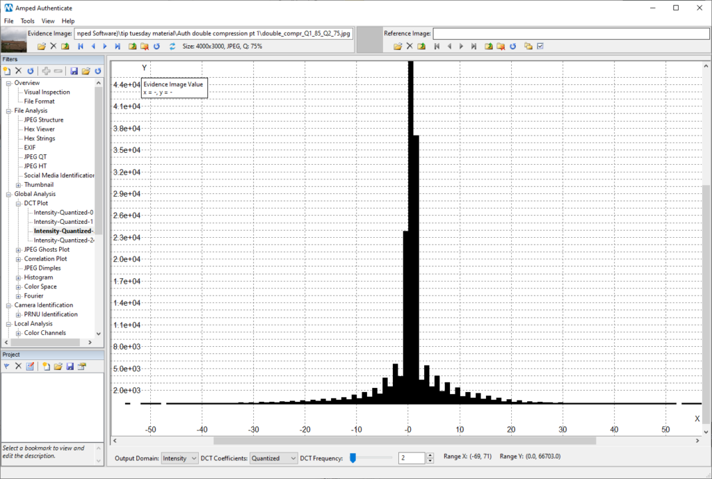
Let’s recap what we showed in the first tip of the series. We’ve seen that manipulated images often undergo two JPEG compressions, one at acquisition time and one to save the result after the manipulation has taken place. Thus, the presence of double compression is of sure interest, as it should trigger the analyst’s attention. We also showed that the JPEG compression algorithm converts pixels to “DCT coefficients” and quantizes them. Therefore double compression implies double quantization. Finally, we showed that Amped Authenticate’s DCT Plot may easily reveal traces of double quantization when the histograms of DCT coefficients become comb-shaped, as shown below.
Today, we’ll mainly focus on the JPEG Ghost Plot, which is just below the DCT Plot in the Filters panel. How the JPEG Ghost Plot works is very easy to explain. It re-compresses the input image one hundred times, at increasing JPEG compression quality (from 1, lowest, to 100, highest). Each time, the compressed image is compared to the evidence image. The mean value of the absolute difference between pixels is plotted. Thus, the plot always has 100 elements on the x-axis (the compression qualities). While the y-axis is devoted to measured differences.
To get practical, let’s compute the JPEG Ghost Plot on a never-compressed image. This is what we get:
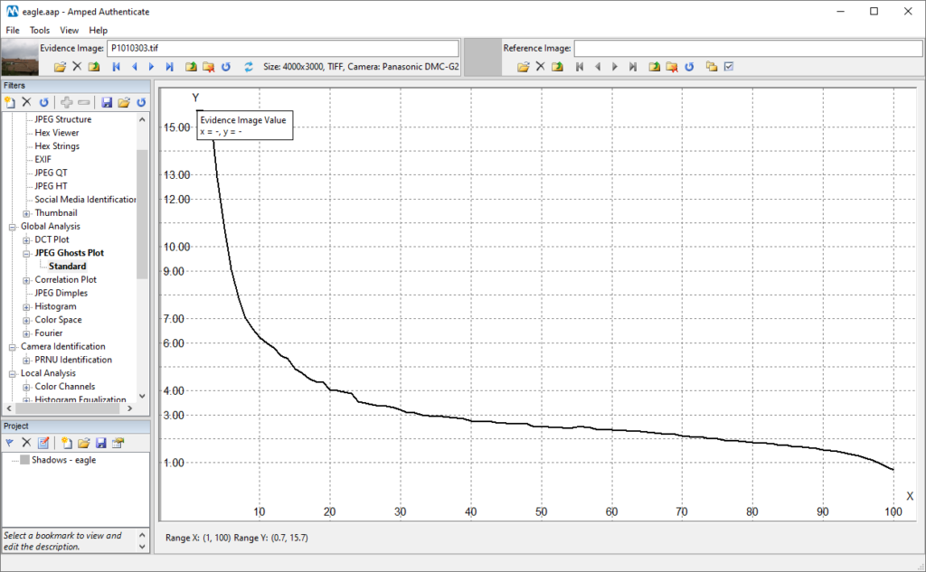
It’s easy to explain: the difference between the evidence image and its re-compressed version is larger for low compression qualities and progressively decreases as the compression quality gets better. You can actually see that, when compression quality is 100, the average pixel difference is smaller than 1, practically unnoticeable.
Okay, that was for a never compressed image. What happens if we analyze a “standard” JPEG image, compressed only once? Below you see the result. But first, notice that that on the top bar there’s written Q: 85%. That information has nothing to do with the JPEG Ghost Plot. It is simply obtained by comparing the image quantization table with the JPEG standard tables. It gives you an estimate of the current JPEG image quality.
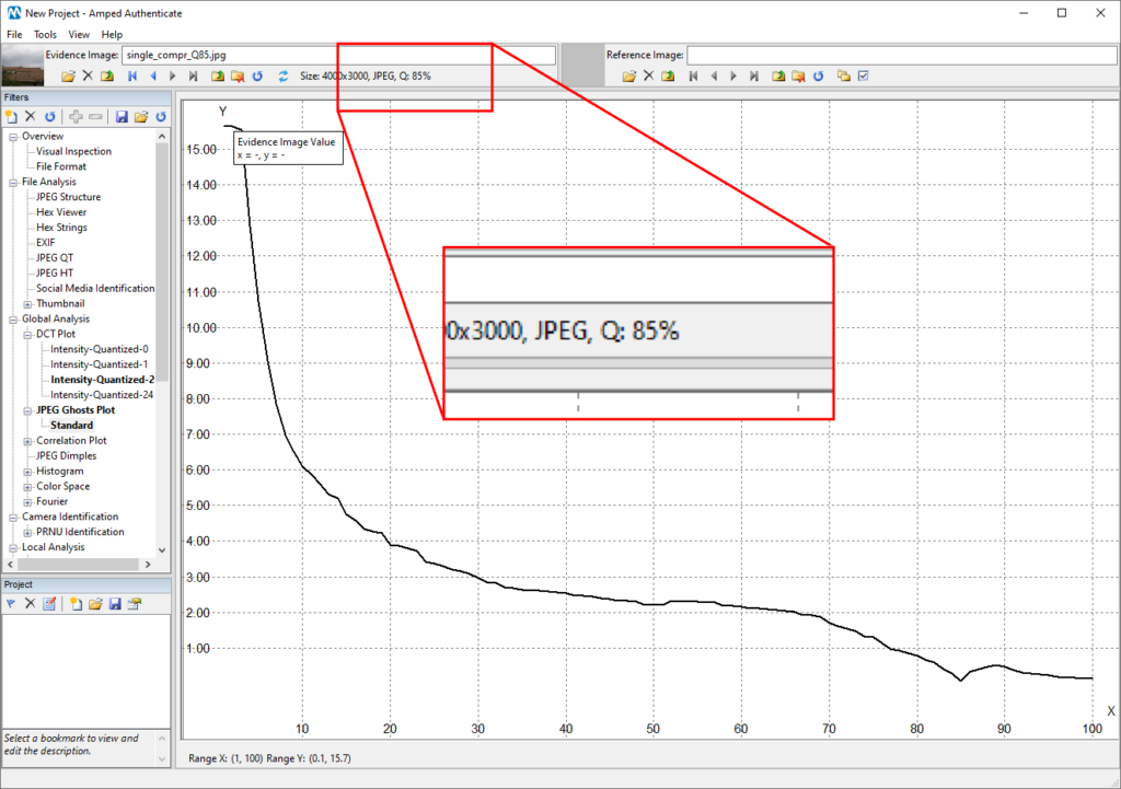
Let’s go back to the plot now. If you look closely, you’ll notice there’s a local minimum before quality 90. Turning on the log-scale (right-click on the plot and select Log Scale Y) and zooming a bit makes it pretty evident. The local minimum is located at quality 85.
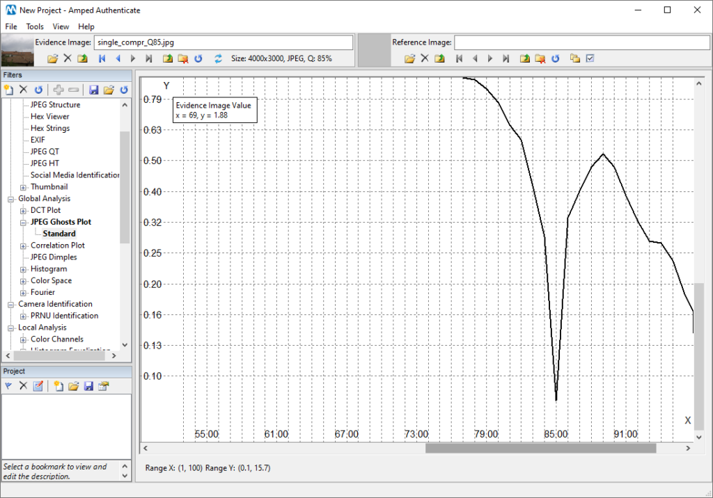
So, when during its compression loop the JPEG Ghost Plot matches the current image quality, the difference suddenly drops, then it returns to the standard behavior. Why is that? It’s because of the JPEG “idempotency property,” which says: re-compressing a JPEG image again with the same parameters will yield identical pixels. Indeed, in the plot above, we see the difference is almost zero at quality 85 (it’s not exactly zero because there are rounding errors in the JPEG compression pipeline).
So, resuming: when we run the JPEG Ghost Plot on a JPEG-compressed image, we expect to find a local minimum at the same quality we read in the top bar, or close to that. I’m saying “or close to that” because, while the filter uses standard JPEG quantization tables for recompressing, cameras often use customized quantization tables. So the idempotency rule only holds approximatively. But that’s not really an issue.
Until now everything was cool. But, in the end, we have just shown that the JPEG Ghost Plot can simply confirm what we already easily see on the top bar: the current JPEG quality of the image.
But what if we load an image that was compressed twice? Let’s re-compress the image we used above at quality 95, and run the filter. Here is the output:
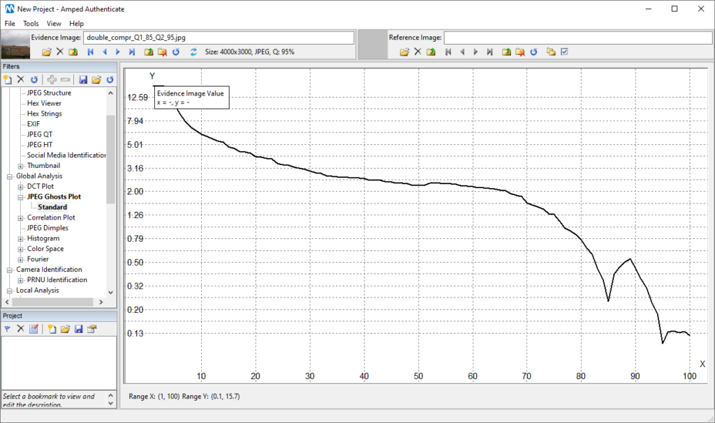
Ha-ha! There are TWO local minima now. One is located at 95, which is the current (i.e., the last compression’s) JPEG image quality. But we also have another one located at 85, which was the previous JPEG compression quality! So the JPEG Ghost Plot filter goes beyond the DCT Plot. Besides telling you there’s a double compression, it allows telling the previous compression quality!
What if we had re-compressed the image at a lower quality, going from 85 (first compression quality) to 75 (second compression quality)? Let’s try:
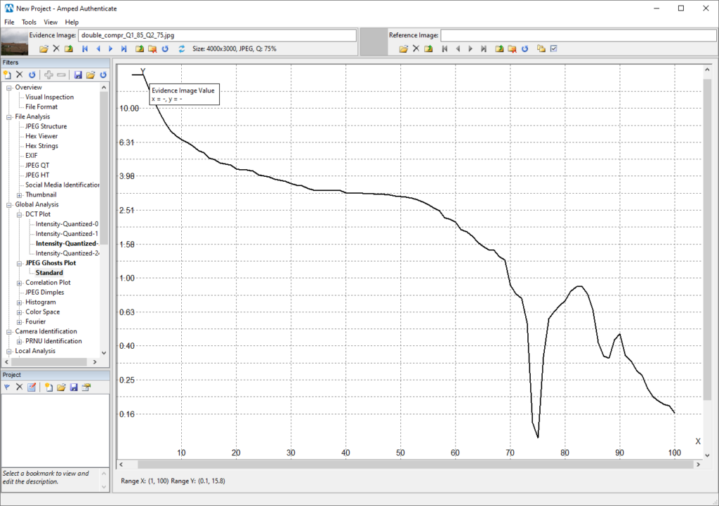
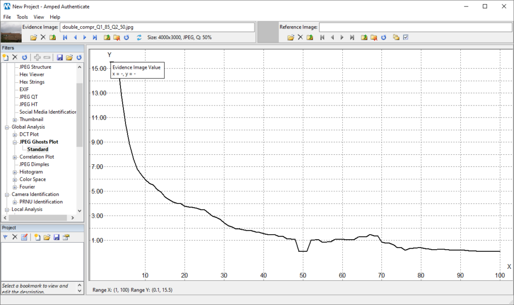
We still find the two peaks, one at the current quality (75) and one roughly at the previous (85). As usual in image forensics, if the last compression is very aggressive it will conceal the traces of past operations (much like someone leaving their marked footprint over that left by somebody else in the past). For example, if we recompress the original image at quality 50, traces of the previous compression disappear:
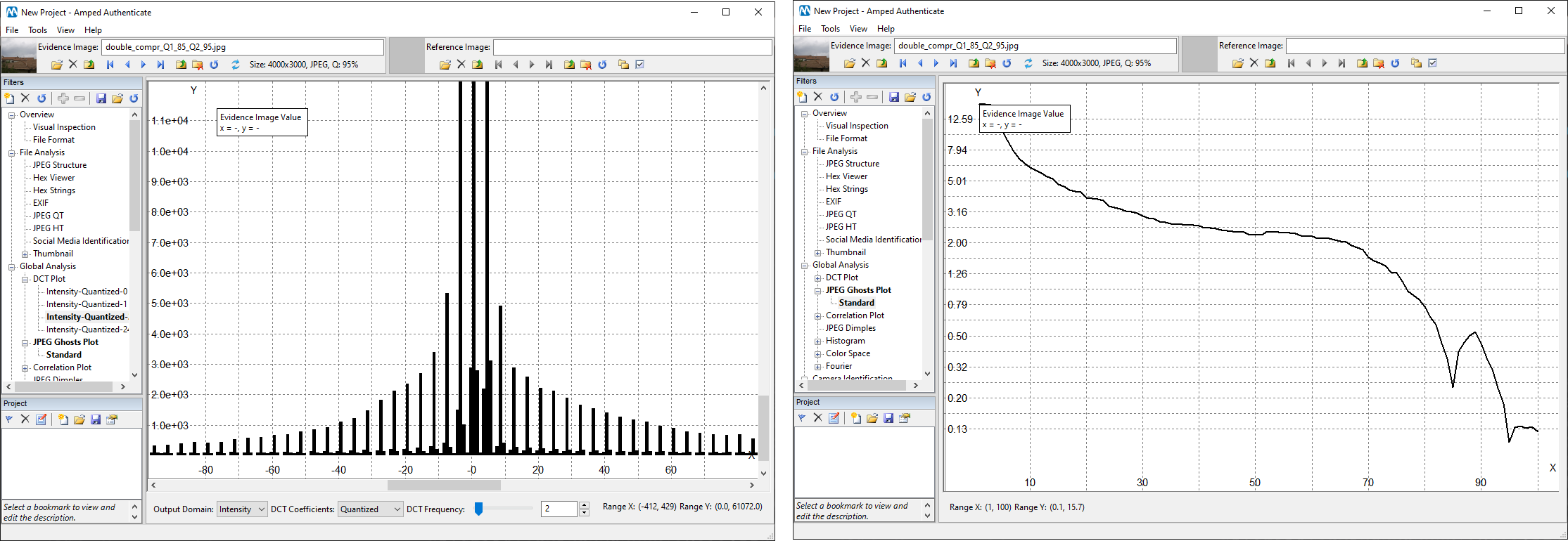
Of course, we always recommend using both the DCT Plot and the JPEG Ghost Plot and jointly interpret and comment on their results. E.g., the combination of plots below provides strong support to the hypothesis that the image was compressed twice, that the latter compression is at a higher quality (since you have empty bins in the DCT Plot) and, more precisely, that the former quality was roughly 85 (since you have a local minimum there in the JPEG Ghost Plot).
And that’s all for this mini-series! You can download the single-compressed and double-compressed images used in this tip from the following link. You can try all of this at home.