Hello, dear Amped blog fellows! This week we’re beginning a mini-series of two tips dealing with one of my favorite topics, image life-cycle investigation! They’re a bit more technical than usual, but I’m sure you’ll enjoy them. Today, we’ll see how we can use Amped Authenticate to look for traces of previous JPEG compressions in your evidence image. In the next tip of the series, we’ll deal with estimating the quality of possible previous JPEG compressions. Keep reading!
During our Amped Authenticate training classes, we always stress that image authenticity verification does not limit to “finding a nice map of forged areas”. Yes, that may be your final target, but if you want your analysis to sound credible, it’s better to corroborate your findings with as much information as possible about the life-cycle of the image. One thing is to say “Hey! This map has a red blob here!”, another thing is to say “This is the hypothesized life-cycle of the image. We have this and this and these elements which are all consistent with the hypothesis, and in such scenario, we find a manipulated part”. Now, the ability to detect a “latent” previous JPEG compression in your image is a key element in image life-cycle reconstruction.
Although the novel and more powerful HEIC compression scheme entered the market recently, JPEG is still the most used format to store images after the acquisition. So, most frequently, when you take a picture with, say, a smartphone or a digital camera, the first JPEG compression occurs at the end of the acquisition phase. That means we normally expect a JPEG image as the “camera original” output file produced by most devices.
Now, when you compress an image with the JPEG algorithm, several steps occur, as indicated by the image below (for the experts: we don’t mention chroma subsampling here as it’s not needed).
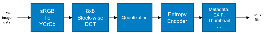
The two key steps of interest to us are the “8-by-8 block-wise DCT” and the “Quantization”. In (very very) simple words, the JPEG algorithm splits the image in non-overlapping 8-by-8 pixel blocks and processes them independently. Each block of pixels is “transformed” with the Discrete Cosine Transform (DCT), which basically “rearranges” the way the information is represented, putting “low frequency” (i.e., smooth transitions) information towards the upper-left part of each block, and “high frequency” (i.e., textures and fine-details) information towards the bottom right. Until this point, no information was removed, so no compression occurred. The trick is that, since the human eye is less sensitive to details, we can be more aggressive in discarding the details and less aggressive in discarding the smooth transitions. That’s obtained by dividing each block by the Quantization Table, whose values grow more and more as we move to the bottom-right part:
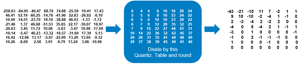
Those that you see on the right-hand are called “quantized DCT coefficients”. As you can see, there are many zeros in the bottom right. These numbers will be arranged and further compressed before being written to file. But we don’t care much for the sake of this tip.
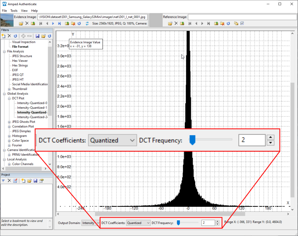
When you receive the image and decode it, you’ll reach a point where you de-quantize those coefficients, which is just the inverse operation. Now, what Amped Authenticate’s DCT Plot filter lets you see, are the histogram of DCT coefficients either before (choose Quantized in the DCT Coefficients menu) or after de-quantization (choose Dequantized). We normally look at the quantized coefficients.
Now, when you choose the DCT Frequency, the filter will collect all coefficients that are in the same position across all 8-by-8 blocks in the image, as visually explained below, and make a histogram of their values.
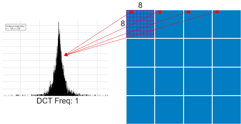
The DCT Frequency number increases in zig-zag order, so numbers follow the order indicated below:

Now, if you load a “normal” image that has been JPEG compressed only once in Authenticate and move to the DCT Plot, here is what you normally find:
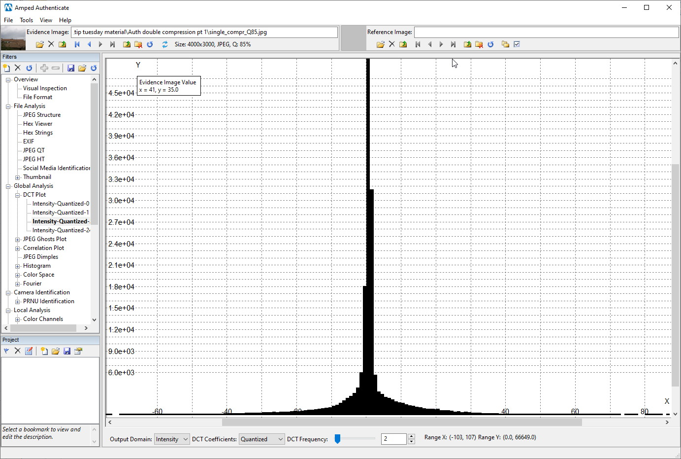
This is the classical, expected distribution of quantized DCT coefficient (for those of you who are curious: it is normally approximated with a Laplacian distribution). As you move to higher DCT frequencies, the quantization table has larger values which coefficients get divided by. So quantized coefficients value is smaller. Thus the distribution gets narrower and narrower around zero, as shown below for frequency 18 (notice on the x-axis that the histogram’s tails stop before reaching 10, while for frequency 2 above they reached 40 and more):

All of this is for a normal, single-compressed image. But what if the image gets re-compressed, e.g. because it has been opened (thus decompressed) in Photoshop and then saved as JPEG (thus re-compressed)? Double compression implies that coefficients undergo the quantization process two times (one per compression). And when you quantize a set of numbers multiple times, strange things happen, which are well exposed by the DCT Plot.
Let us take the image used above, which was JPEG compressed once at quality 85 (you could see this quality written in the top bar), and re-compress it at quality 95. Here is how the DCT Plot looks for the double compressed image:
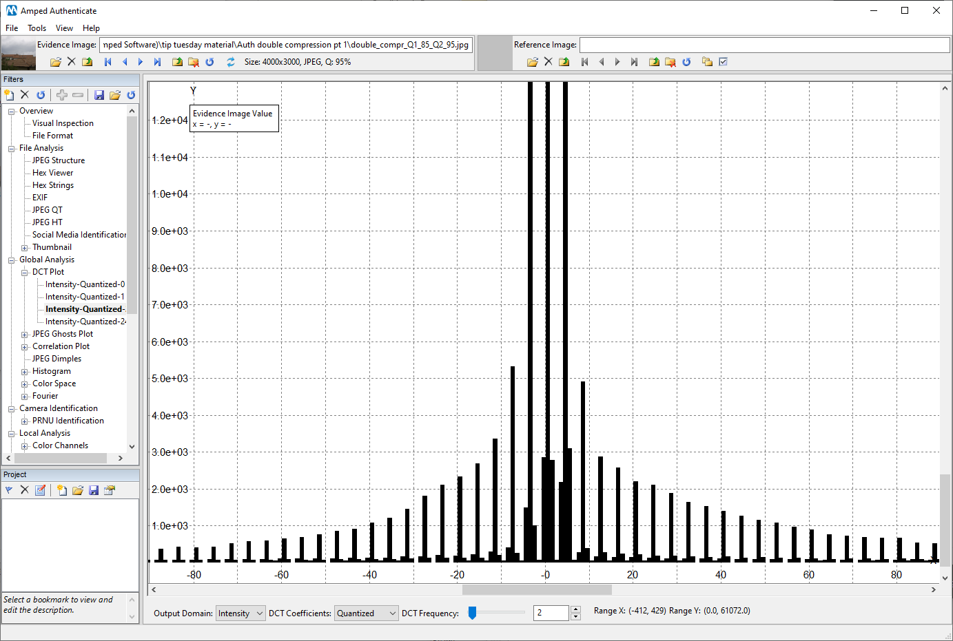
That periodic, comb-shaped histogram indicates that DCT coefficients underwent a double quantization. It reasonably means the image has been JPEG-compressed twice. The alternation between peaks and almost-empty bins also tells us something more. For that frequency, the value in the quantization table used for the second compression was smaller than that used for the former compression. Which means: the last compression was probably at a higher quality than the former one (the example above in indeed obtained with first compression at quality 85 and second at quality 95).
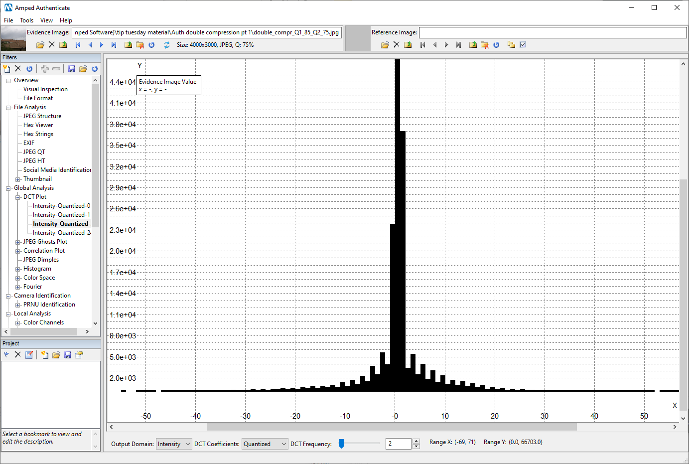
And what if the quality decreased in the second compression? We should be able to still see periodic peaks in the histogram. But the valleys are no longer empty, they do contain some values. Here is what we obtain by taking the original 85-quality image and re-compressing it at quality 75:
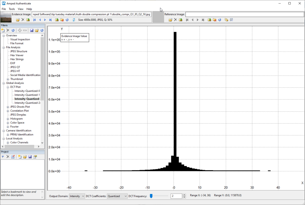
Of course, if the last compression is very aggressive, it will just conceal previous traces. Here is the DCT Plot if we recompress at quality 50 instead: no periodic peaks appear anymore.
Let’s recap a bit, then! If you have an image whose DCT Plot looks smooth for all frequencies, or perhaps has an irregular shape for some frequencies but without the presence of a regular alternation of peaks-and-valleys, then we say we don’t find evidence of double compression with this tool.
But if you observe a DCT Plot with an evident peak-and-valley behavior (even for a few frequencies only!), we can reasonably say the image underwent two JPEG compressions. Which is something we don’t expect for camera original images (except for some devices that, curiously, produce native images with such artifacts, such as older iPhones).
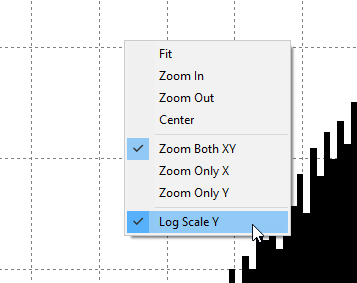
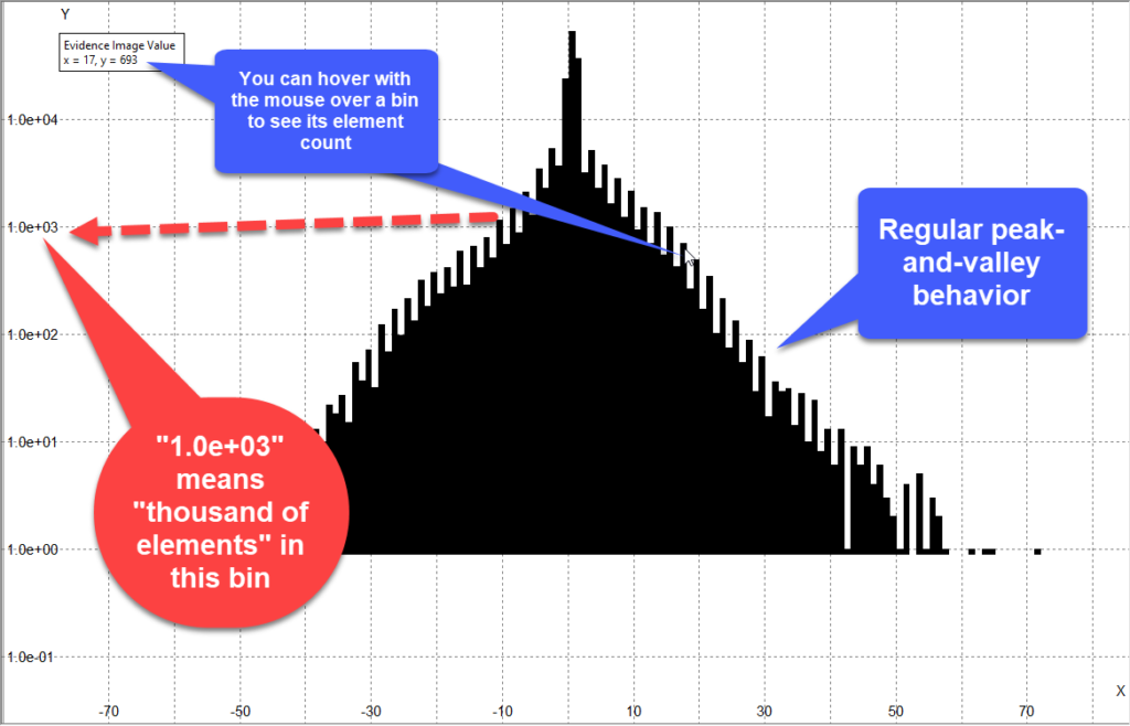
Remember that you can right click on the plot and choose to view values in the Log-scale, as explained in this past tip.
This could boost detectability of peaks. Keep in mind that you should draw conclusions only when bins of the histogram contain a sufficiently large number of elements (hundreds, at least)
That’s it for today! In the next tip of the series, we’ll see how we can dig even deeper into investigating the compression history of an image.
Before we say goodbye, here’s a gift for you: you can download the single-compressed and double-compressed images used in this tip from the following link, so you can try all of this at home.