We hope you’re aware of the big news. A few weeks ago, an extraordinary Amped FIVE update rolled out bringing Speed Estimation 2d filter into the software. We’ve dedicated a blog post to explain what the filter does and how to use it. We recommend that you read that post before going on with this one. Hereafter, indeed, we’ll be explaining how the filter works, how we compute the speed estimation and the uncertainty. Happy reading!
Topics
- Working hypotheses for the Speed Estimation 2d filter
- Challenges to speed estimation from digital videos
- Dealing with perspective
- Handling uncertainties in the process
- Measuring speed for steering vehicles
Introduction to Speed Estimation
Let’s start with a formulation of the problem. We have a video of a vehicle, which could be getting closer or farther from the camera. Also, we have timing information for each frame. Finally, we want to compute the vehicle’s speed.
Now, the formula for computing the average speed of an object is taught in middle school. You just need to divide the traveled distance by the time needed to cover it. However, in our problem, we have a few issues that complicate the scenario:
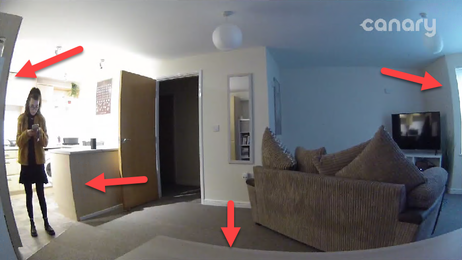
- Optical distortion: most surveillance cameras are equipped with fisheye lenses in the attempt to capture as much scenery as possible. However, these lenses introduce the so-called barrel distortion. As a consequence, things that are rectilinear in the real world appear curved in the captured image. This needs to be fixed before carrying out any kind of spatial measurement on the video, including speed estimation. You can find more info about correcting optical distortion in this post.
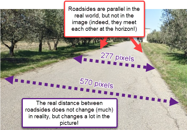
- Perspective distortion: lines that are parallel in the real world are not so in the picture because of perspective. As an obvious consequence, the amount of “real” space between two pixels in two different portions of the frame is different.
- Uncertainty: it is often impossible to know the position of the object at a pixel level, e.g. the video may be blocky or it may have a limited definition. Also the timing accuracy of frames cannot be taken for granted.
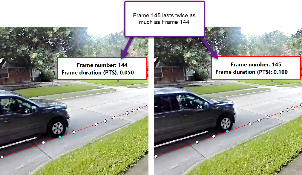
- Variable Frame Rate Videos: it is quite common to find videos where the time distance between frames is not constant at all. This must be taken into account of course.
How did we tackle these issues?
Dealing with Perspective
Our strategy is to move the problem to a 2D space where distances are known (more or less it means working with an orthophoto of the scene). In order to do so, we need two elements:
- The vertices of a known rectangular object lying on the road surface. By knowing how a rectangular object looks like in the image allows us to compute a pixel transformation that will make the rectangle’s sides parallel again. This produces a so-called “rectified” image, just as we do in the Correct Perspective filter. However, for speed estimation we need one more information…
- The length of both sides of the rectangle. This is needed to be able to take measurements over the rectified image.
Speed Estimation 2d Filter
This whole process is made very easy in the Speed Estimation 2d filter. The user draws the grid and provides its sizes (see the previous post for more details).
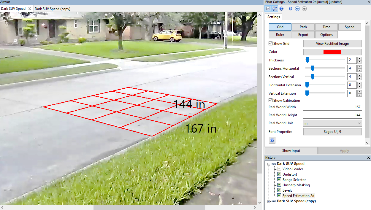

If there is no rectangular reference object laying on the road surface to be used, then we can’t carry out the analysis. Of course, if the camera is still there unchanged, we could go back to the scene and put a checkerboard or any other rectangular element on the ground. Then, we use that video to draw the grid, and copy-paste the so-configured Speed Estimation 2d filter over our evidence video. That’s fine!
Remove Perspective
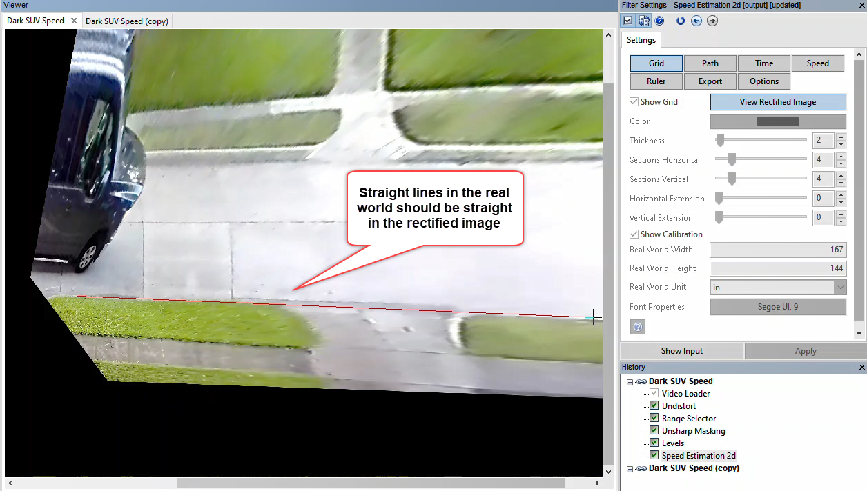
Ok, using the grid data we are able to “remove perspective”. You can click on the View Rectified Image button to have a look at the planar image. When viewing the image in this mode, you can click and drag to draw a line. This is useful to check that straight lines are actually straight in the rectified image. If this is not the case, it could be due to suboptimal optical distortion correction, or a mistake in drawing the grid.
It is important that you understand that errors in drawing the grid or in distortion removal will have an influence on the correctness of the estimated speed. Once you’re done with your speed analysis, you may create some copies of the filter, try to “perturb” a bit the grid selection, and evaluate the impact that such changes have on your estimates.
Dealing with Uncertainty
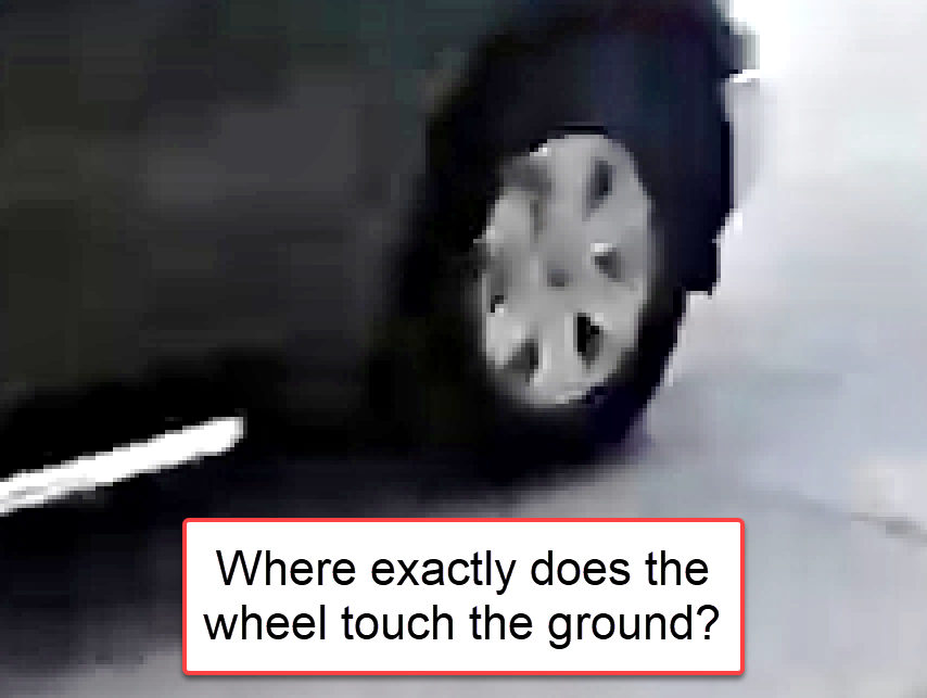
Now that perspective is gone, we need to track the object’s trajectory. As explained in the previous post, this is achieved by using the Path tool and clicking, for each frame, over the contact point between the wheel and the ground.
It is important that only points on the ground (i.e., where the wheel touches the road) are considered when drawing the path. In fact, our rectification only works for that specific plane. This is why, in the rectified image, the car looked “more natural” in its bottom part and completely distorted on its top.
The Pixel Uncertainty Parameter
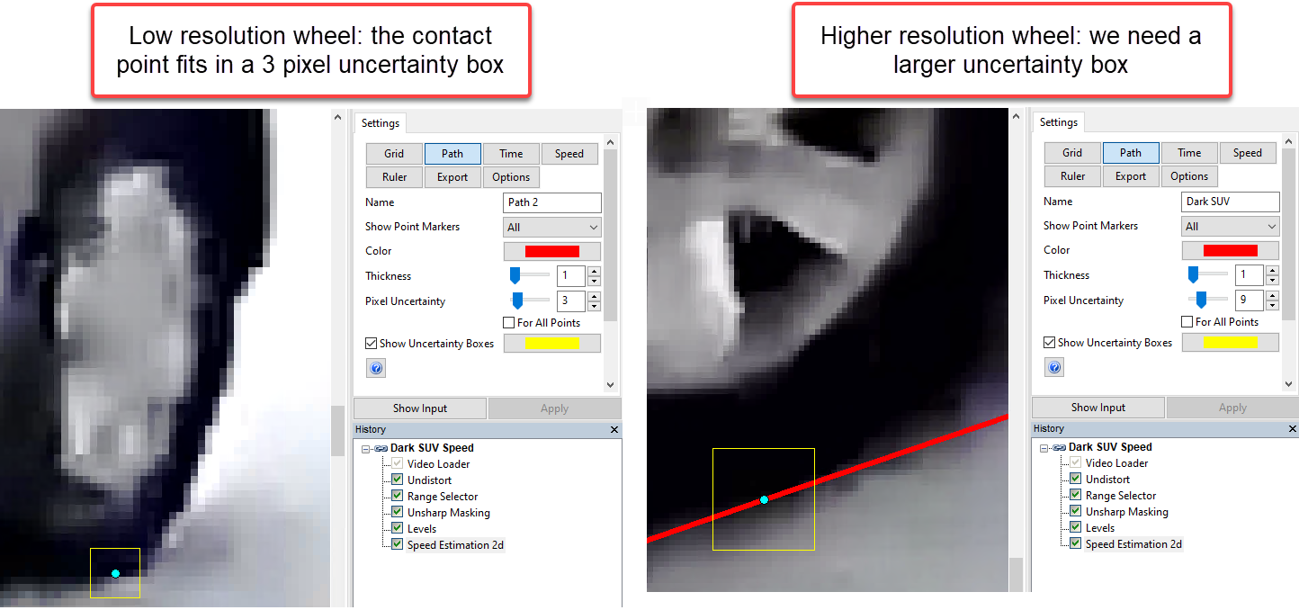
As you know from the previous post, we are not forced to specify a single pixel. Thanks to the Pixel Uncertainty parameter we can draw a box that surely contains the contact point.

Although it may sound a bit counter-intuitive, for a given video we will likely need larger boxes when the car is closer to the camera and smaller boxes when it’s farther away. This is well explained in the example below. Remember, indeed, that we don’t need to factor perspective in our box selection. That will be automatically considered by the estimation algorithm!
How do these uncertainty boxes contribute to the speed estimation? For a couple of connected points P1 and P2, we have two boxes, B1 and B2. The central distance is the point-to-point distance between P1 and P2. We then compute the minimum and maximum possible distances between all points contained in B1 and B2. Noticeably, this computation is carried out on the rectified image, where these boxes are no longer squares! This is better explained visually below.

Since the difference between the central and minimum distances is not necessarily the same as the difference between the central and maximum distances, we play it safe and define the distance uncertainty as:

Speed Estimation Between Two Neighboring Frames
Now, let’s imagine for now that we’re only interested in speed estimation between two neighboring frames (which is usually not a good idea, as we’ll see later). The uncertainty on speed has been defined above. How about time?
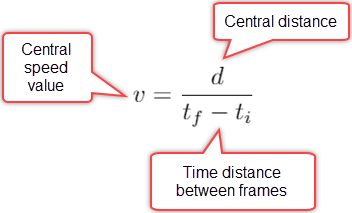
In the Time tool, we can choose the timing source for the video and provide a time uncertainty. We already discussed in last week’s post some principles to be considered for setting this value. In our case, we’ll set it to 2.5 milliseconds. Now, we have a distance with its uncertainty and a time duration with its uncertainty. The central value of the speed is obviously obtained by:
How about the uncertainty? We need to apply a rule which says that, when combining the product between two measurements, the relative uncertainty of the product is obtained by summing the relative uncertainty of the measurements. To get the relative uncertainty we simply need to divide the measurements by the uncertainty value. So, we have for distance and time, respectively:
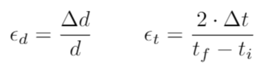
Which then gives us the relative uncertainty of speed by a simple sum:
And to turn the speed uncertainty from relative to absolute, we simply need to multiply it by the central speed value:

… and we’re done!

What we’ve seen above works for computing the speed and its uncertainty between TWO points. For a more stable and reliable speed estimation, however, it is recommended to use many frames.
When you try computing the speed between two neighboring frames, you’ll likely end up with large uncertainties. This is known and, to some extent, “wanted”. You shouldn’t get the impression that a video can give you precise estimates of the “instantaneous speed”. It’s much, much safer to compute the average speed on a larger number of frames.
Walk the Line
Once we’ve drawn the full vehicle’s path we want to consider, it should be quite evident whether it’s traveling in a straight line or it’s turning. Depending on this condition, we should use different ways of computing the speed.
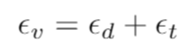
If the vehicle travels in a straight line, we can just consider the distance between the first and last points of the path. We call this “Minimal Distance”. In the example below, the traveled distance, speed, and uncertainties depend only on the positions of the first and last points of the trajectory.
If the vehicle is turning, things aren’t as simple. We need to compute the length of the whole trajectory. We call this “Path Length” – keeping into account each contact point’s uncertainty (remember you can set different uncertainty box sizes for each point).
Speed Estimation 2d uses the most possible prudent way of combining measurements. It computes the total distance summing the central distance value between all N points, and for the uncertainty, it sums all the uncertainties.

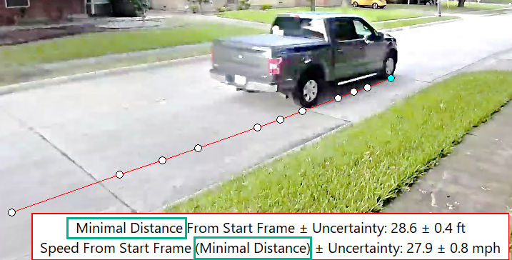
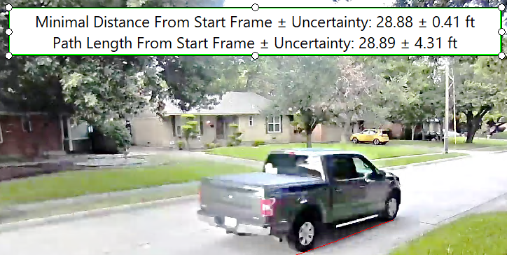
That means you’ll get larger uncertainty ranges for both traveled distance and speed when using the Path Length macros. Here’s a comparison for the example shown above. Notice how larger the traveled distance (green box) and speed (red box) uncertainties are when computed with the Path Length approach compared to the Minimal Distance!
If you’re not sure whether the vehicle is traveling on a straight line, plot both the distance computed with the Minimal Distance method and the one used with the Path Length. If their central value is the same (up to a certain tolerance), it means that the car is traveling straight. In our example above, the Minimal Distance and Path Length central values are indeed very close.
Conclusion
And that’s it! We’ve shared the most important bits of how the Speed Estimation 2d filter works. Before concluding, we’d like to remember some important caveats:
- Speed estimation should be carried out on the original footage, since transcoding or screen capturing could interfere with timing metadata and thus reduce speed analysis accuracy.
- You must compensate for optical distortion before carrying out the analysis.
- The reference grid object must lay on the street. If there’s nothing to be used for reference, and you can’t go back to the scene and take a recording of it with the same setup and settings, then you can’t use Speed Estimation 2d.
- Remember that if the vehicle is travelling on a straight line, macros based on Minimal Distance are preferable. Nevertheless, you’ll need to draw the full path, setting a contact point for every frame.
- Although we provide macros for computing the speed between neighboring frames, we recommend computing the average speed on several frames. However, it is typically better to avoid including frames where the car is excessively distant from the camera, as they would likely increase the uncertainty by a large amount.
We hope all of the above makes sense to you! If you need more information or have questions, feel free to contact our support team!
Stay tuned and don’t miss the next posts! You can follow us on LinkedIn, YouTube, Twitter, and Facebook: we’ll post a link to every new article so you won’t miss any!